Method Comparison
In general, an X% confidence interval should capture the population parameter of interest in X% of samples. In this blog post, I perform a 2 × 4 × 2 factorial simulation study to compare..
Posted by Alfred Prah on March 17, 2020 · 7 mins read
Introduction
Coverage probability is an important operating characteristic of methods for constructing interval estimates, particularly confidence intervals. We care about it because it is the proportion of the time that the interval contains the true value of parameter of interest. It can be defined as the long run proportion of intervals that capture the population parameter of interest. Conceptually, one can calculate the coverage probability with the following steps:- generate a sample of size N from a known distribution
- construct a confidence interval
- determine if the confidence captures the population parameter
- Repeat steps (1) - (3) many times. Estimate the coverage probability as the proportion of samples for which the confidence interval captured the population parameter
1. True, underlying distribution
- standard normal
- gamma(shape = 1.4, scale = 3)
- method of moments with normal
- method of moments with gamma
- kernel density estimation
- bootstrap
- sample min (1st order statistic)
- median
- Sample size, N = 201
- Outside the loop estimation
Generating Data
The true, underlying distribution is either the Standard Normal distribution with mean = 0 and standard edeviation = 1 or a Gamma distribution with shape = 1.4 and scale = 3.
generate_data <- function(N,dist,sh,sc){

  if(dist=="norm"){

    return(rnorm(N)+4)

  }else if (dist=="gamma"){

    return(rgamma(N,shape=sh,scale=sc))

  }

}
Estimating the Confidence Interval
As mentioned earlier, there are 4 models we will be investigating in this experiment: method of moments with normal, method of moments with gamma, kernel density estimation and boostrap.To calculate the parameter of interest for each of these models, we will generate sample that have the same sample size as the data in the last step, and then calculte the parameter of interest(min/median). We can repeat this step several times but for the purposes of this blog post, I'll limit the replicates to 5000. Now let's define the 90% confidence interval of the parameter of interest as the middle 90% of the sampling distribution of the parameter of interest. The lower confidence limit for a parameter of interest is the 0.05 quantile.
The upper confidence limit for a median is the 0.95 quantile.
estimate.ci <- function(data,mod,par.int,R=5000,smoo=0.3){

  N<- length(data)

  sum.measure <- get(par.int)


  if(mod=="MMnorm"){

    mm.mean <- mean(data)

    mm.sd <- sd(data)

    samp.dist <-NA

    for(i in 1:R){
      sim.data <- rnorm(N,mm.mean,mm.sd)

      if(par.int=="median"){

        samp.dist[i] <- median(sim.data)

      }else if(par.int=="min"){

        samp.dist[i] <- min(sim.data)

      }


    }

    return(quantile(samp.dist,c(0.05,0.95)))


  }else if(mod=="MMgamma"){

    mm.shape <- mean(data)^2/var(data)

    mm.scale <- var(data)/mean(data)

    sim.data <- array(rgamma(N*R,shape=mm.shape,scale=mm.scale),dim=c(N,R))

    samp.dist <- apply(sim.data,2,FUN=sum.measure)

    return(quantile(samp.dist,c(0.05,0.95)))


  }else if(mod=="KDE"){

    ecdfstar <- function(t,data,smooth){

      outer(t,data,function(a,b){pnorm(a,b,smooth)}) %>% rowMeans

    }


    tbl <-data.frame(

      x = seq(min(data)-2*sd(data),max(data)+2*sd(data),by=0.01)

    )


    tbl$p <-ecdfstar(tbl$x,data,smoo)

    tbl <- tbl[!duplicated(tbl$p),]


    qkde <- function(ps,tbl){

      rows <- cut(ps,tbl$p,labels=FALSE)

      tbl[rows,"x"]

    }


    U <- runif(N*R)

    sim.data <- array(qkde(U,tbl),dim=c(N,R))

    samp.dist<-apply(sim.data,2,sum.measure)

    return(quantile(samp.dist,c(0.05,0.95)))

    #qqplot(data,sim.data)

    #abline(0,1)


  }else if(mod=="Boot"){

    sim.data <- array(sample(data,N*R,replace=TRUE),dim=c(N,R))

    samp.dist<-apply(sim.data,2,sum.measure)

    return(quantile(samp.dist,c(0.05,0.95)))

  }

}
Capturing the Parameter
The confidence interval will capture the true paramter if the lower confidence limit is less than the true parameter, and the upper confidence limit is greater than the true parameter. To execute the "parameter-capturing" process, let's create a function that tests whether the confidence interval captured the true parameter or not. The function will return a 1 if the confidence interval captured the true parameter or a 0 otherwise.
capture_par <-function(ci,true.par){
  1*(ci[1]
Coverage Probability
It is now time to calculate the Coverage Probability, the long run proportion of intervals that capture the population parameter of interest. To calculate the coverage probability for our different models, we will compute the mean of "captures" by repeating the above steps:generate_data %>% estimate.ci %>% capture_par
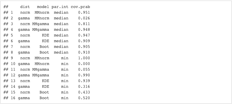
For the purposes of this blog post, I repeat this 1000 times. The values obtained as the means of captures are our Coverage Probability. The coverage probabilities for our various combinations are shown in the table below:
N <- 201

shape.set <- 1.4

scale.set<-3


true.norm.med <- qnorm(0.5)

true.norm.min <- mean(apply(array(rnorm(N*10000),dim=c(N,10000)),2,min))

true.gamma.med <- qgamma(0.5,shape=shape.set,scale=scale.set)

true.gamma.min <- mean(apply(array(rgamma(N*10000,shape=shape.set,scale=scale.set),dim=c(N,10000)),2,min))


simsettings <- expand.grid(dist = c("norm","gamma"),model=c("MMnorm","MMgamma","KDE","Boot"),par.int=c("median","min"),cov.prab=NA,stringsAsFactors = FALSE,KEEP.OUT.ATTRS = FALSE)


for (k in 1:nrow(simsettings)){

  dist1 <-simsettings[k,1]

  model1 <-simsettings[k,2]

  par.int1 <- simsettings[k,3]


  if(dist1=="norm" & par.int1=="median"){

    true.par1 = true.norm.med+4

  }else if(dist1=="norm" & par.int1=="min"){

    true.par1 = true.norm.min+4

  }else if(dist1=="gamma" & par.int1=="median"){

    true.par1 = true.gamma.med

  }else if(dist1=="gamma" & par.int1=="min"){

    true.par1 = true.gamma.min

  }


  cover <- NA

  for(sims in 1:1000){

    cover[sims] <- generate_data(N,dist1,1.4,3) %>% estimate.ci(mod=model1,par.int=par.int1,R=5000,smoo=0.3) %>%      capture_par(true.par=true.par1)

  }

  simsettings[k,4] <- mean(cover)


}

simsettings

write.csv(simsettings,"simulation_results.csv")
Analysis/Conclusion
From the table above, we can observe the following:- For the Normal distribution, the Coverage Probability of the Min is very small if it is estimated with the method of moments with gamma
- For the Gamma distribution, the Coverage Probabilities of the Min and Median are very small if we use method of moments with normal to estimate them
- The bootstrap method generally generates a low Coverage Probability for the Min