Introduction

In this blog post, we explore a concept known as the “Coverage Probability”. Coverage probability is an important operating characteristic for constructing the interval estimates of statistical methods, particularly Confidence Intervals. To explore this concept, I will perform a simulation to calculate the coverage probability of the 95% confidence interval of the median when computed from through the Maximum Likelihood Estimation, MLE. For the purposes of this blog post, let’s define the 95% confidence interval of the median to be the middle 95% of sampling distribution of the median. Similarly, the 95% confidence interval of the mean, standard deviation, etc. is the middle 95% of the respective sampling distribution. In the same light, let’s define the coverage probability as the long run proportion of intervals that capture the population parameter of interest. Conceptualy, one can calculate the coverage probability with the following steps: 1. generate a sample of size N from a known distribution 2. construct a confidence interval 3. determine if the confidence captures the population parameter 4. Repeat steps 1 - 3 many times. Estimate the coverage probability as the proportion of samples for which the confidence interval captured the population parameter.

Generating Data

First, using “rnorm”, let’s generate a sample from a Standard Normal Distribution of size N = 201.

 

N <- 201 

pop.mean = 0 

pop.sd = 1 

true.parameters <- c(N,mean = pop.mean, sd = pop.sd) 

generate_data <- function(parameters){ 

  data=rnorm(parameters[1],parameters[2],parameters[3]) 

}

Using MLE to estimate the distribution

 

est.mle <- function(data) { 
 
  mean.mle <- mean(data) 
 
  sd.mle <- sd(data) 
 
  return(c(length(data),mean.mle,sd.mle)) 
 
}  

   true.parameters %>% generate_data %>% est.mle

Results:

201.00000000
0.03067752
1.00997949

We see that the the mean and standard deviation for the generated sample are about 0 and 1, respectively.

Calculating the Confidence Interval for the Median

We now get to use the mean and standard deviations we estimated through the MLE to generate a sample that we will compute the median of, by running 5000 simulations.
As mentioned earlier, the 95% confidence interval of the median will be assumed to be the middle 95% of the sampling distribution of the median.
The lower and upper confidence limits for the median are the 0.025 and 0.975 quantiles, respectively.

 

boot.meds.ci <- function(parameters){ 

  R <- 5000 

  sample.meds <- NA 

  for (i in 1:R){ 

    sample.meds[i] <- parameters %>% generate_data()%>% median 

  } 

  quantile(sample.meds,c(0.025,0.975)) 

}

The True Median

The median of a Standard Normal Distribution is 0. A Confidence Interval will capture the median if the lower confidence limit is less than zero or the upper confidence limit is greater than zero. The chunk of code below returns a 1 if the confidence interval captured the true median or a 0 if the confidence interval failed to do so.

 

capture_median <- function(ci){ 
 
  1*(ci[1]<0 & 0 
}

Coverage Probability

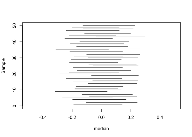
As mentioned earlier, the Coverage Probability is an important operating characteristic of methods for constructing interval estimates, particularly confidence intervals. Wikipedia defines it as the proportion of the time that the interval contains the true value of interest.

The plot above shows the 95% confidence interval of 50 samples. Intervals in black capture the population parameter of interest; the ones in blue do not. In this instance, the coverage probability is ~ 49/50.

Coverage Probability of the Median

Taking the 95% confidence interval calculated for 5000 samples, we can compute the Coverage Probability as the proportion of samples for which the Confidence Interval captured the true value of the Median:

 

M <- 5000 
 
captures <- rep(NA, M) 
 
for(i in 1:M){ 
 
  captures[i] <- true.parameters %>% generate_data %>% est.mle %>% boot.meds.ci %>% capture_median 
 
}
 
capture_prob <- mean(captures) 
 


capture_prob

Answer: 0.9868
The Coverage Probability for the 5000 simulations we run is ~ 98%. Ideally, a 95% confidence interval will capture the population parameter of interest in about 95% of the sample. Our simulations did slightly better than 95%.

← Previous Post Next Post →