Central Limit Theorem (R stats)
The central limit theorem is an important computational short-cut for generating and making inference from the sampling distribution of the mean..
Posted by Alfred Prah on March 13, 2020 · 4 mins read
Introduction
The central limit theorem is an important computational short-cut for generating and making inference from the sampling distribution of the mean. The central limit theorem short-cut relies on a number of conditions, specifically:
- Independent observations
- Identically distributed observations
- The pre-existence of the Mean and variance
- A sample size large enough for convergence
In this simulation study, I use QQ-plots to graphically compare the sampling distribution of the mean generated by simulation to the sampling distribution implied by the central limit theorem. For the purposes of this simulation, let’s treat the mean and variance as known values and use the actual population parameters and the population mean and variance instead of sample estimates.
To generate a sample, I initialize the parameters (size of sampling distribution, central location and scale of the skew-normal distribution) that do not change at the beginning.
Parameters that do not change
- R <- 5000
- location <- 0
- scale <- 1
Comparison
To pave the way for comparison, I conduct a 4 x 4 factorial experiment to compare the distributions in the QQ-plots. The first factor is the sample size, with N = 5, 10, 20, and 40. The second factor is the degree of skewness in the underlying distribution. The underlying distribution is the Skew-Normal distribution.
The Skew-Normal distribution has three parameters: location, scale, and slant. When the slant parameter is 0, the distribution reverts to the normal distribution. As the slant parameter increases, the distribution becomes increasingly skewed. In this simulation, slant will be set to 0, 2, 10, 100. Set location and scale to 0 and 1, respectively, for all simulation settings.
par(mfrow = c(4,5))


for (slant in c(0, 2, 10, 100)) {


  ## Plot distribution

  if (slant == 0) {

    curve(dsn(x, xi = location, omega = scale, alpha = slant), -3, 3, main= "Distribution", xlab = "", ylab = paste0("Slant = ", slant), xaxt = "n", yaxt = "n", cex.main = 1.5, cex.lab = 1.5)

  }

  else {

    curve(dsn(x, xi = location, omega = scale, alpha = slant), -3, 3, xlab = "", ylab = paste0("Slant = ", slant), xaxt = "n", yaxt = "n", cex.lab = 1.5)

  }


  for (N in c(5, 10, 20, 40)) {

     delta <- slant/(sqrt(1+slant^2))

     pop_mean <- location+scale*delta*(sqrt(2/pi))

     pop_sd <- sqrt(scale^2*(1-(2*delta^2)/pi))

     Z <- rnorm(R)

     sample_dist_clt <- Z*(pop_sd/sqrt(N)) + pop_mean

     random.skew <- array(rsn(R*N, xi = location, omega = scale, alpha = slant), dim = c(R,N))

     sample_dist_sim <- apply(random.skew, 1, mean)


    # QQ plot

    if (slant == 0){

        qqplot(sample_dist_sim, sample_dist_clt, asp = 1, main = paste0("N = ", N), xlab = "", ylab = "", xaxt = "n", yaxt = "n", xlim = c(-1.6,2), ylim = c(-1.6, 2.2), cex.main = 1.5, cex.lab = 1.5)
      abline(0,1)

      }

    else {

       qqplot(sample_dist_sim, sample_dist_clt, asp = 1, xlab = "", ylab = "", xaxt = "n", yaxt = "n", xlim = c(-1.6,2.2), ylim = c(-1.6, 1.6), cex.lab = 1.5)
      abline(0,1)

    }

  }

}
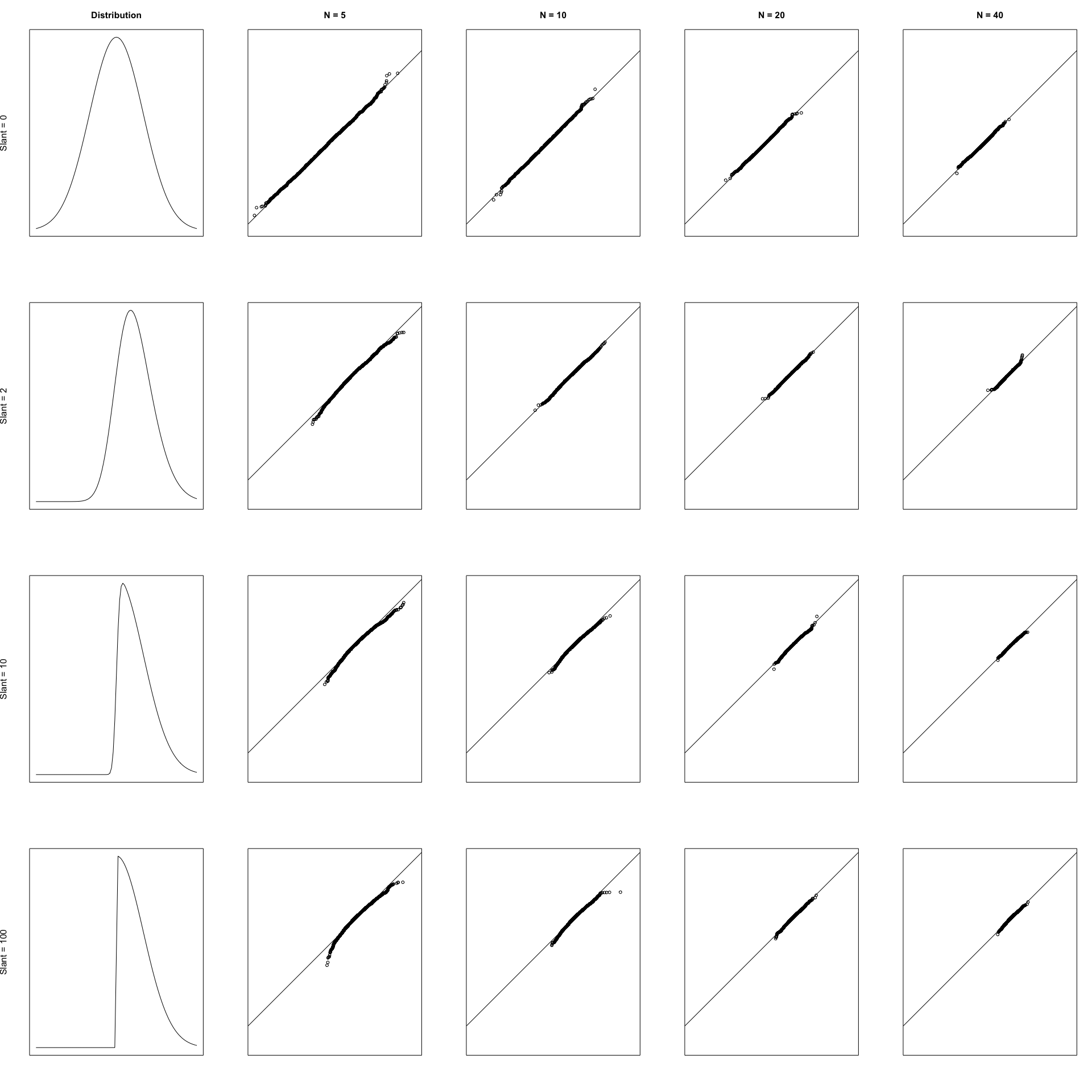
Observations
From the plots above, we can conclude the following:- As the sample size increases, the plotted points fall along the line y=x more precisely
- There will be more deviation in the tails of a plot as the slant increases